Quadrangle Inequality trick for dynamic programs
Application: Given an ordered list of keys with frequencies, build a binary search tree on those keys which minimizes the average query cost.
This note has been updated in January 2024. We corrected one error in our implementation. See the paragraph right before the implementation for more detail.
Formal definition
In the 1970’s a technique was discovered by Knuth and generalized in the 1980’s by Yao, which permits to speedup any dynamic program of a particular form and particular property.
We illustrate the technique on the following problem. Informally, we want to construct a binary search tree, over given keys, which minimizes the average query cost.
Formally, we are given some keys numbered from $1$ to $n$, together with frequency vectors
\[\begin{array}{cccc} &\beta_1& &\beta_2& &\ldots& &\beta_n \\ \alpha_0& &\alpha_1& &\alpha_2 & &\alpha_{n-1}& &\alpha_{n} \end{array}\]such that $\beta_i$ is the frequency of queries of the $i$-th key, $\alpha_i$ is the frequency of a query between the $i$-th and the $i+1$-th key. Here we consider fictitious keys indexed $0$ and $n+1$.
A binary search tree is a rooted tree where
- every inner node is associated to a key index $i$ and has weight $\beta_i$,
- inner nodes have a left and a right subtree,
- every leaf has weight $\alpha_i$.
Such a tree has to satisfy the usual left-to-right ordering according to the indices of the keys.
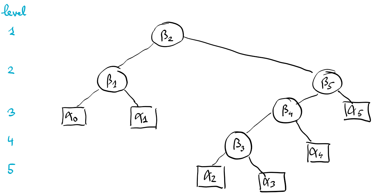
The cost of a tree is called the weighted path length and is defined as the sum over all nodes of the weight of the node multiplied with the level of the node in the tree.
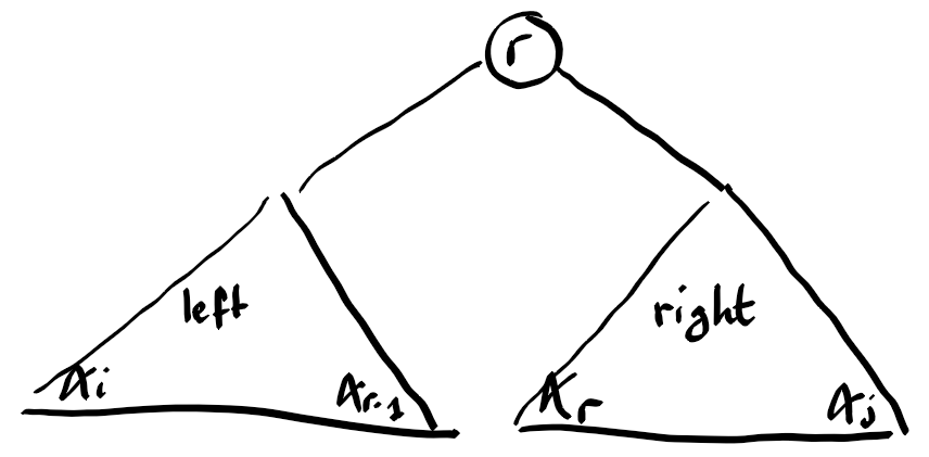
An optimal search tree can be computed using dynamic programming. For every $0\leq i\leq j\leq n$ consider the problem of building the optimal search tree for queries restricted to be strictly between the $i$-th key and the $j+1$-th key. We call it the problem restricted to $(i,j)$, or subproblem $(i,j)$. We consider the following values.
- $C[i,j]$ is the cost of the optimal search tree
- $W[i,j]$ is the total frequency of the restricted problem. It is $\alpha_i +\beta_{i+1}+ \alpha_{i+1} + \ldots+\beta_{j}+\alpha_j$.
- $R[i,j]$ is the root of the optimal search tree. It is defined only for $i < j$ and satisfies $i+1 \leq R[i,j] \leq j$.
These values lead to the following dynamic program. For the base case $i=j$ we have
\[C[i,i] = W[i,i] = \alpha_i\]and for $i < j$ we have
\[C[i,j] = W[i,j] + \min_{i+1\leq r\leq j} (C[i,r - 1] + C[r,j]) \\ R[i,j] = \textrm{argmin of above expression}.\]The optimal search tree of the subproblem contains a root $i+1\leq r\leq j$, which motivates the minimum expression above. The addition of $W[i,j]$ comes from the fact that by attaching the left and right subtrees under the root $r$, the level of all their nodes increases by $1$. Since root $r$ has level one, the weight $\beta_r$ has to enter the cost of the tree as well.
This leads to a time complexity of $O(n^3)$, because we have $O(n^2)$ variables, each being the minimum over $O(n)$ alternatives.
Improvement to $O(n^2)$
Donald Knuth made this clever observation 50 years ago, that the root does not have to be searched within the full range. The following range is enough:
\[R[i,j - 1] \leq R[i,j] \leq R[i + 1,j], \tag{1}\]and therefore
\[C[i,j] = W[i,j] + \min_{R[i,j-1]\leq r\leq R[i+1,j]} (C[i,r - 1] + C[r,j]).\]This would mean that the time needed to compute $R[i,j]$ is proportional to $R[i,j-1] - R[i+1,j] + 1$. Summing up over all $i,j$ with fixed difference $j-i$, we obtain a telescopic sum of value $O(n)$. Hence the total time complexity is $O(n^2)$.
A general framework
Such an improvement applies under some condition to any dynamic program of the form
\[C[i,i] = 0 \\ C[i,j] = W[i,j] + \min_{i<k\leq j} (C[i,k-1]+C[k,j]) \:\:\textrm{ for } i < j.\]This dynamic program generalizes the previous one, but for the special case $\alpha=0$. This simplifies the presentation.
The dynamic program above, in essence depends on the matrix $W$. And it is the structure of $W$, which permits the above mentioned improvement. Two properties of $W$ are essential.
- $W$ satisfies the quadrangle inequality (denoted QI for short) if for every $a\leq b\leq c\leq d$ we have
- $W$ is monotone on the lattice of intervals if for every $a\leq b\leq c\leq d$ we have
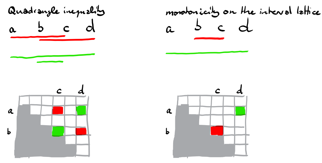
Note: the quadrangle inequality is also called the Monge property. And it is enough that it is satisfied for $b=a+1,d=c+1$, because then it is satisfied as well for larger $b,d$.
F. Frances Yao shows that whenever $W$ satisfies the two properties, then the inequality (1) holds, which allows to solve the dynamic program in quadratic time.
This holds for a variety problems, such as
- Optimal binary search tree for given query frequencies
- Given sets of strings $S_1,\ldots,S_n$, compute the multi-set of strings obtained by concatenating a string from $S_1$ with a string from $S_2$ and so on and finally concatenating with a string from $S_n$. Every concatenation between two strings generates one unit of cost. The goal is to perform the task at minimum cost.
- Given $n$ points in convex positions, and an integer $m < n$, compute a convex polygon using $m$ among the $n$ points which has longest perimeter.
The proof idea
For the formal proof we refer to Yao’s paper, referenced at the bottom of this document. In a nutshell it consists of the following steps.
Lemma 1 If $W$ satisfies QI and is monotone on the lattice of intervals, then $C$ also satisfies QI.
Proof
The proof of $$ C[a,c] + C[b,d] \leq C[b,c] + C[a,d] \:\:\textrm{ for all } a\leq b\leq c\leq d $$ is by induction on the difference $d-a$. When $a=b$ or $c=d$, both sides of the inequality are identical. This establishes the base case $d-a\leq 1$. The induction step considers two cases. **Case** $a<b=c<d$: In this case the inequality to show becomes the inverse triangular inequality $$ C[a,b]+C[b,d] \leq C[a,d] \:\:\textrm{ for all } a<b<d. $$ Let $k$ be the minimizer for the expression of $C[a,d]$, i.e. $C[a,d]=C_k[a,d]$, using the notation $C_k[a,d] := W[a,b] + C[a,k-1]+C[k,b]$. If $k\leq b$ we have $$ \begin{array}{rll} C[a,b]+C[b,d] &\leq C_z[a,b] + C[b,d] &\text{(by opt. of C[a,b])} \\ &= W[a,d] + C[a,k-1]+C[k,b] + C[b,d] \\ &\leq W[a,d] + C[a,k-1] + C[k,d] &\text{(by ind. hyp., using a<k)}\\ &= C[a,d]. &\text{(by choice of k)} \end{array} $$ The case $k > b$ is similar. **Case** $a<b<c<d$: Let $k,\ell$ be such that $$ C[b,c] = C_k[b,c] \textrm{ and } C[a,d] = C_\ell[a,d]. $$ If $\ell\leq k$ we have $$ \begin{array}{rll} C[a,c] + C[b,d] &\leq C_\ell[a,c] + C_k[b,d] &\text{(by opt.)} \\ &= W[a,c] + W[b,d] +C[a,\ell-1] + C[k,c] + C[b,k-1]+C[k,d] \\ &\leq W[b,c] + W[a,d] +C[a,\ell-1] + C[k,c] + C[b,k-1]+C[k,d] &\text{(by QI of W)} \\ &\leq W[b,c] + W[a,d] +C[a,\ell-1] + C[b,k-1]+C[k,c] + C[\ell,d] &\text{(by ind. hyp.)} \\ &= C_k[b,c] + C_\ell[a,d] \\ &= C[b,c] + C[a,d]. \end{array} $$ The case $\ell > k$ is similar. And this concludes the proof.Lemma 2 If $C$ satifies QI, then
\[K[i,j] \leq K[i,j+1] \leq K[i+1,j+1] \textrm{ \:\:for } i\leq j,\]where $K[i,j]$ is the minimizer of the minimum expression in the definition of $C[i,j]$, and for convenience we denote $K[i,i]=i$.
Proof
It holds by definition of $C$ when $i=j$. To show the first inequality in case $i < j$, we will show for $a < b\leq c < d$ $$ \left[ C_c[a,d] \leq C_b[a,d] \right] \Rightarrow \left[ C_c[a,d+1] \leq C_b[a,d+1] \right]. \tag{2} $$ By the quadrangle inequality we have $$ C[b,d]+C[c,d+1] \leq C[c,d] + C[b,d+1]. $$ And if we add $W[a,d]+W[a,d+1]+C[a,b-1]+C[a,c-1]$ to both sides we obtain $$ C_b[a,d]+C_c[a,d+1] \leq C_c[a,d]+C_b[a,d+1] $$ which shows the implication (2). The proof for the second inequality is similar.Implementation in Python
We said earlier that the minimizer for the recursive expression for $C[i,j]$ ranges between $i+1$ and $j$, but can be restricted to the range between $K[i,j - 1]$ and $K[i + 1, j]$. This means that the actual range has to be in the intersection of these ranges, hence the use of max in the range expression for variable $k$ in the code below.
def dyn_prog_Monge(W):
    """ Solves the following dynamic program for 0 <= i < j < n

    C[i,i] = 0
    C[i,j] = W[i,j] + min over i < k <= j of (C[i,k-1] + C[k,j])
    K[i,j] = minimizer of above

    :param W: matrix of dimension n times n
    :assumes: W satisfies the Monge property (a.k.a. quadrangle inequality) and monotonicity in the lattice of intervals
    :returns: C[0,n-1] and the matrix K with the minimizers
    :complexity: O(n^2)
    """
    n = len(W)
    C = [[W[i][i] for j in range(n)] for i in range(n)] # initially C[i,i]=W[i][i]
    K = [[j for j in range(n)] for i in range(n)] # initially K[i,i]=i

    # recursion
    for j_i in range(1, n): # difference between j and i
        for i in range(n - j_i):
            j = i + j_i
            argmin = None
            valmin = float('+inf')
            for k in range(max(i + 1, K[i][j - 1]),  K[i + 1][j] + 1):
                alt = C[i][k - 1] + C[k][j]
                if alt < valmin:
                    valmin = alt
                    argmin = k
            C[i][j] = W[i][j] + valmin
            K[i][j] = argmin
    return C[0][n-1], K
References
The first reference is the original paper introducing the quadratic time algorithm. There were many followup researchs, which are summarized in the second reference.
- Knuth, D. E., Optimum binary search trees, Acta Informatica, 1(1), pages 14–25, 1971.
- Yao, F. Frances. Efficient dynamic programming using quadrangle inequalities. Proceedings of the twelfth annual ACM symposium on Theory of computing. 1980.
- Nagaraj, S. V. Optimal binary search trees, Theoretical Computer Science, 188(1–2), pages 1-44, 1997.
- Our implementation of the actual code to build the optimal binary search tree