PC Trees
A data structure representing all permutations satisfying constraints of the form: for a given set $S\subseteq\{0,1,\ldots,n-1\}$ the elements of the permutations on $\{0,1,\ldots,n-1\}$ have to be consecutive in circular manner.
Warning
We propose a simplified implementation which does not have the optimal time complexity. When restricting with a set $S$, the complexity won’t be in $O(|S|+p)$, where $p$ is the length of the terminal path (see below for definition), but in time $O(|S|+d)$, where $d$ is the total degree along the vertices of the terminal path.
To improve the implementation, one would need to replace the Python sets in P-nodes by a more sophisticated data structure.
However the performance still allows to solve the following problem in linear time in the size of the matrix. Given a matrix with 0,1 entries, the goal is to find, if possible, a permutation of its columns, such that in every row the 1’s are consecutive.
Acknowledgement
The little we know about PC-trees, we got it from the excellent ESA’2021 paper by Fink, Pfretzschner and Rutter.
Introduction
Suppose you want to shoot a film and need to decide in which order to film the different scenes, such that ideally every actor participates in consecutive scenes. Formally you are given a binary matrix $M\in\{0,1\}^{n\times m}$ and want to know if there is a permutation of its columns, such that in the resulting matrix every row matches the regular expression $0^\star1^\star0^\star$. Such a matrix is said to have the consecutive ones property (C1P for short). There exists a circular variant of this problem, where rows are in addition allowed to match the expression $1^\star0^\star1^\star$. In this variant, the column indices are considered to belong to the integers modulo $n$, namely $\mathbb Z_n$. These variants are essentially equivalent, since adding a column with only zeros reduces the non-circular variant to the circular one.
This problem has been introduced in 1899 by an archeologist named Petrie, who tried to place tombs on a timeline,assuming that ornaments observed in each tomb appeared at some moment in history and eventually became out of fashion. This situation could be modeled as the C1P-problem for a matrix $M$, where columns correspond to tombs, rows to ornaments, and a 1 in the matrix indicates the presence of an ornament in a particular tomb. In 1976 Booth and Luecker presented a data structure, called PQ-tree, which permits to solve the problem in linear time. Later in 1999 Shih and Hsu proposed a similar data structure called PC-tree, which was initially designed to embed planar graphs, and which solves the circular variant of the problem. According to Fink, Pfretzschner and Rutter, this data structure is easier to implement and more efficient.
Informal introduction
Given a permutation $\sigma$ on ${\mathbb Z}_n$ and a set $S \subseteq {\mathbb Z}_n$, we define the signature of $S$ in $\sigma$ as the binary string $b$, such that $b_i = 1$ if $\sigma_i \in S$ and $b_i=0$ otherwise. For example, for
         sigma = (7, 8, 3, 9, 4, 1, 2, 3, 0)
         and S = {7, 8,       4, 1}
the signature is  1  1  0  0  1  1  0  0  0.
We say that $S$ is consecutive in $\sigma$ if its signature is of the form $0^\star1^\star0^\star | 1^\star0^\star1^\star$ (denoted as a regular expression). For example, for the above mentioned permutation $\sigma$, the set $\{1,4,7,8\}$ is not consecutive, but the set $\{0,2,3,7\}$ is consecutive and so is the set $\{1,4\}$.
For a given collection of sets $S_1,\ldots,S_k$ we want to maintain in a compact data-structure the set of all permutations for which each of the sets is consecutive.
For such a data structure, we want to be able to produce one of these valid permutations, and also to add a new set $S$ to the collection. The later operation will restrict the set of permutations stored in the data structure. We call this operation a restriction by $S$.
Other operations are possible, such as returning the number of valid permutations or choosing uniformly at random one of the valid permutations. But to keep this note simple, we do not consider these features.
This data structure will be represented by a tree, where the leafs are all the elements of ${\mathbb Z}_n$. Any depth first traversal of the tree will visit the leafs in some order. Inner nodes impose some restriction on the order to visit neighboring nodes, hence restricting the set of possible permutations.
Formal definition
A PC-tree is a tree consisting of $n$ leafs labeled from $0$ to $n-1$ and inner nodes of type P or C. C-nodes have a fixed order on their neighbors, while P-nodes have not. For simplification we assume that no inner node has degree 2.
Such a tree represents in compact form permutations on $\{0,1,\ldots,n-1\}$. These permutations can be obtained by a depth first traversal of the tree (DFS), starting from say the leaf labeled 0, and listing all leaf labels along the traversal. When exploring the neighbors of a P-node, we can explore them in arbitrary order. But when exploring the neighbors of a C-node, we can explore them either in clock-wise or counter-clock-wise order starting from the neighbor that lead to this C-node. These choices lead to all permutations encoded by the tree.
Example
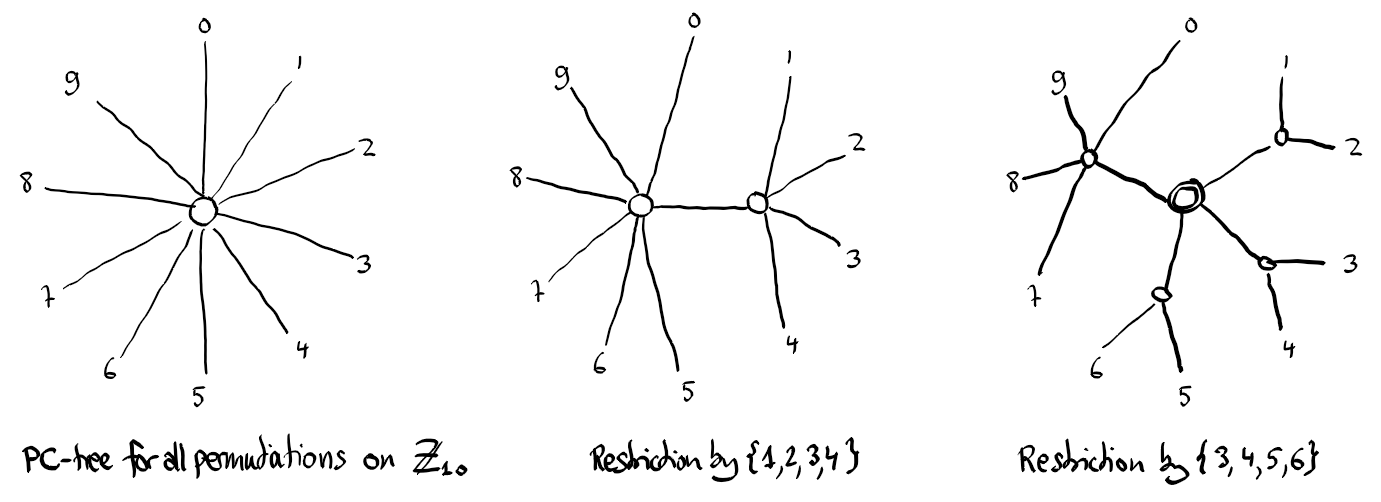
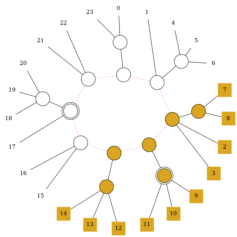
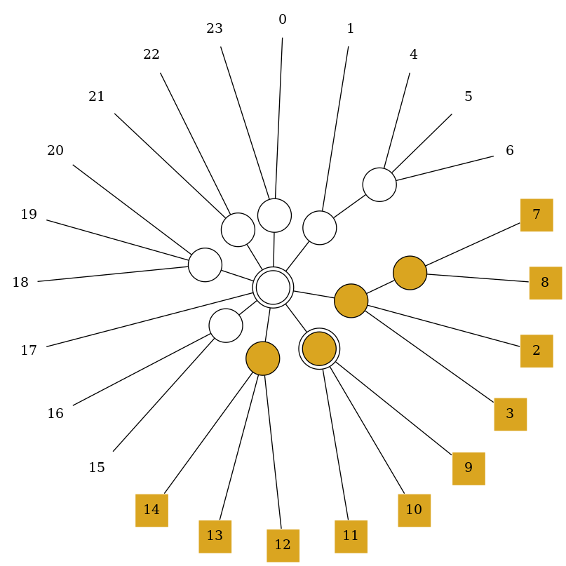
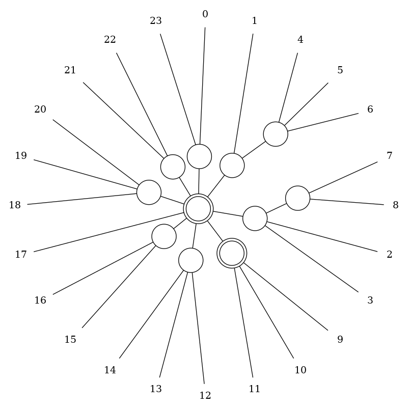
The left tree represents all permutations on $\{0,1\ldots,9\}$. P-nodes are depicted as circles with simple border, while C-nodes have a doubled border, as in the right tree. The middle tree represents all permutations keeping the set $\{1,2,3,4\}$ consecutive. We say that the permutations are restricted by the set $\{1,2,3,4\}$. In the right tree we restricted also by the set $\{3,4,5,6\}$.
Restriction
The restriction of a PC-tree by a set $S$, transforms the tree such that it forbids permutations where elements of $S$ are not consecutive. The restriction is done by transforming the tree using the following steps, which are explained in the sequel of this note.
- Test cardinality If the cardinality of $S$ is 0,1,n-1 or n, the restriction will not modify the tree, and the procedure ends here.
- Label the nodes A leaf $i$ is full if $i\in S$ and empty otherwise. The labels propagate further to the inner nodes, which are labeled full, empty or partial. (full definition below)
- Identify terminal path The smallest subtree $T$ spanning all the partial nodes is identified. If $T$ is not a path, then the restriction is not possible and the procedure is aborted. If $T$ is a path, we call it the terminal path.
- Split nodes All vertices in $T$ are disconnected from each other. Partial nodes in $T$ are split into a full and an empty node.
- Simplify The resulting list of nodes is modified as follows: Degree 1 nodes are replaced by their neighbor and C-nodes are replaced by their list of neighbors.
- Reconnect nodes The list of nodes is connected to a new C-node.
- Clean up The data structure needs to be cleaned such that all variables used for the restriction are again in their initial state. This action needs to be conducted also when the restriction procedure is aborted.
High level example
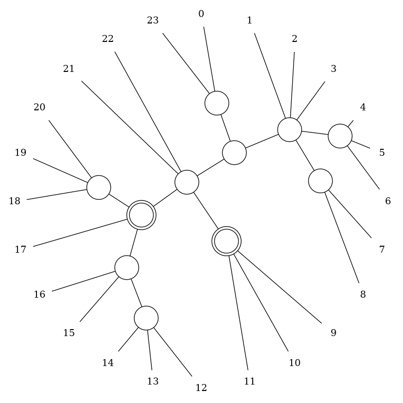
Suppose we have the following PC-tree.
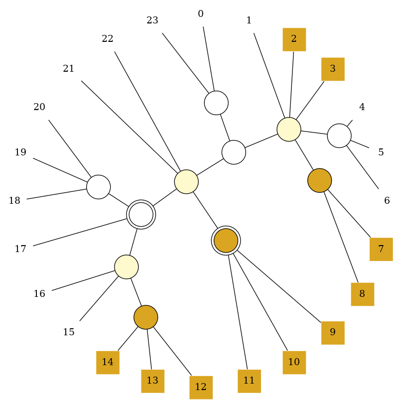
Now we want to restrict it by the set $\{2,3,7,8,\ldots,14\}$. First we label the nodes as empty, partial or full. This is done starting from the leafs and propagating towards the inner nodes.
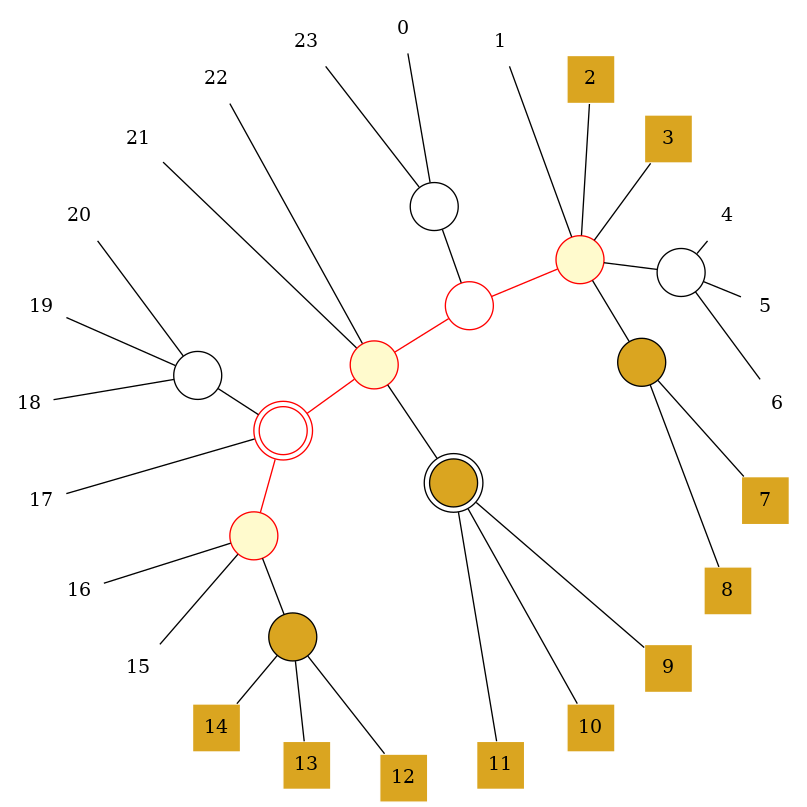
Then we identify the terminal path connecting all partial nodes.
Now we remove the edges between the nodes along the terminal path, resulting in a list of nodes (forming a forest). Partial nodes from this list are split such that the original nodes are connected to all empty neighbors, while the new nodes are connected to all full neighbors. This results in a circular list of nodes.
The list is simplified, in the sense that degree 1 nodes are replaced by their neighbor and C-nodes by their neighbor list.
A new C-node is created attaching all nodes from the list.
Finally the tree is cleaned, in the sense that all nodes are labeled empty as they were initially.
Structure of the implementation
We have 3 classes: Leaf, P_node and C_node which all inherit from a super-class Node. Nodes have
- a pointer to a
parentnode, which encodes the orientation of the tree towards a root node. For the root node this attribute isNone. - an identifier
ID. This integer is used to represent the tree in text form. - an integer
full_counter, which keeps track of the number of full neighbors. - inspectors
is_fullandis_partial, which determine the node label, according to thefullCounter`. - method
signal_fullused by a neighbor to signal to this node that it (the neighbor) became full. - method
cleanto reset the full_counter. - methods to
attachanddetachnodes with each other. These methods maintain the parent pointer.detach_bilateralremoves an edge between two nodes, by detaching them on both endpoints.attach_neighborsattaches a node to all its neighbors.
A PC_tree is a class which has
- an initializer with a given number
n - a method
restrictwhich restricts the tree by a given set $S\subseteq \{0,1,\ldots, n-1\}$ - a method
representwhich returns a canonical representation of the tree in form of a list of list. Each inner list represents an inner node, and contains a characterPorCfor the type, its identifier and its list of neighbors in lexicographical minimal order. This list can optionally end with the identifier of the parent node. - a method
frontierwhich returns a valid permutation represented by the tree. With some little work it is possible to extend this method to make it select uniformly at random a valid permutation, or to return the lexicographically smallest one.
These 3 subclasses have in common
- a method
to_signalwhich for a full node returns the neighbor to which a signal needs to be send. For a leaf it is just the inner node to which the leaf is attached to, and for inner nodes it is the unique neighbor which hasn’t be signaled.
P and C-nodes have in common
- an inspector
is_splittablewhich tests if the node is splittable, which means roughly that its full neighbors are or can be made adjacent. - a method
splitwhich returns a new node with only the full neighbors. - an attribute
neighbors, which is a sequence for the C-node and a set for the P-node. In addition C-node has an attributefirst_fullwhich is the first full neighbor to have signaled to this node. It is used as a starting point to explore the neighbors in order to find a maximal interval of full neighbors.
C-nodes have a method flip, which inverts the order of the neighbors.
In addition we have an exception called Infeasible which is raised whenever we find out that the restriction fails.
Labeling
Inner nodes are labeled as follows. Initially all inner nodes are empty. When all but one neighbor of a node become full, then the node becomes also full. This process is implemented by a signaling procedure using a queue, starting with the full leaves. Every node in the queue signals to its unique non-full neighbor that it became full, and is removed from the queue. And when this neighbor has enough full neighbors, then it becomes full and joins the queue.
Identifying the terminal path
This is trickiest part of the procedure. We would like the complexity to be linear in the maximum distance between partial nodes. So a tree traversal to compute the distances is too costly. In principle the tree is not rooted, but if we maintain an orientation towards a root, then we can obtain the aimed time complexity.
Formal problem
We are given a rooted tree on a vertex set $V$. There is a function $f : V \mapsto V \cup \{ \bot \}$, which returns the ancestor for every non-root vertex, and returns $\bot$ for the root vertex. In addition we are given a set of vertices $S$, which we call the seeds. The goal is to decide if there is a simple path $P$ containing all vertices $S$. Here simple means that $P$ contains no cycles.
Let $a$ be the lowest common ancestor of all vertices in $S$, which is also called the apex. Denote by $S \rightarrow a$ the union of all paths connecting $a$ with every vertex in $S$. So the problem consists in deciding if $S \rightarrow a$ is a path or not. We aim for an algorithm with complexity $O (| S \rightarrow a |)$.
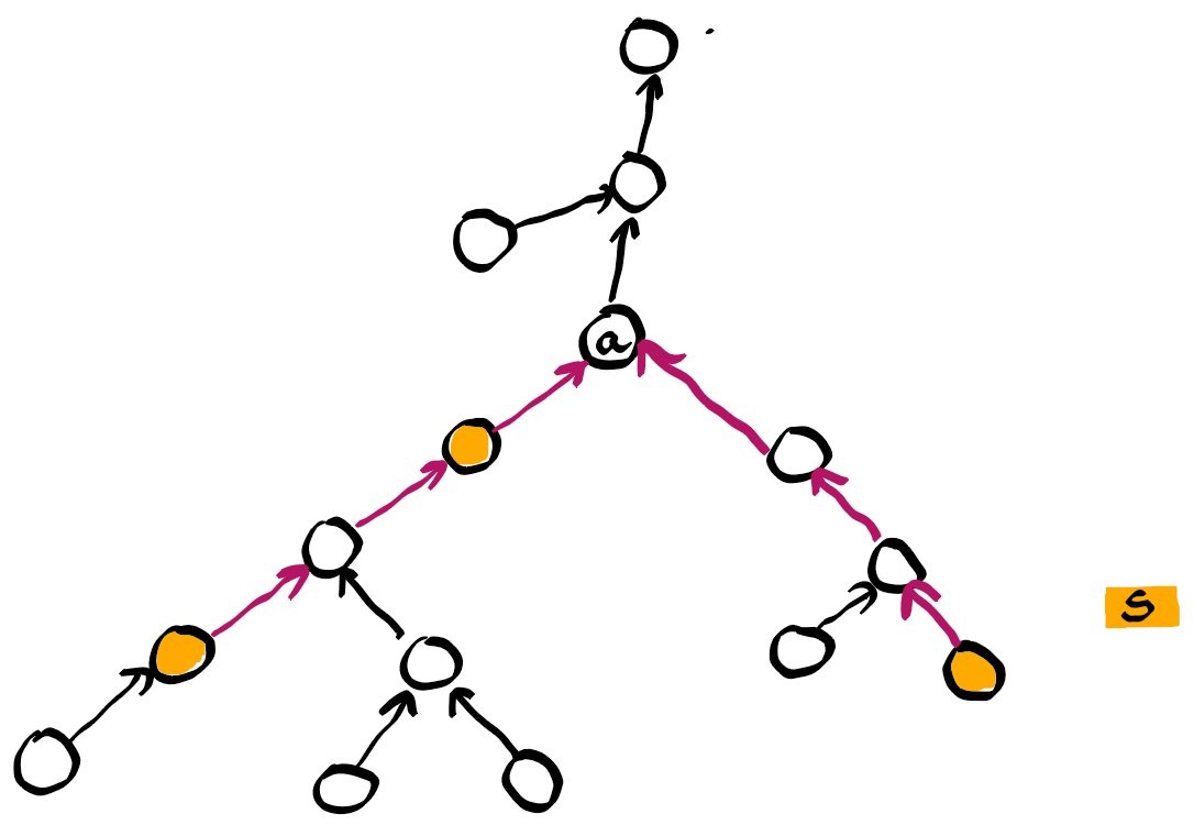
For a yes-instance, the resulting path is completely described by the apex $a$ and one or two vertices in $S$, which are the extreme points of the path and called tails.
In the particular case when $S$ is a singleton set, we can answer yes, because this single vertex forms itself the resulting path. So from now assume $| S | \geqslant 2$.
The rough idea of the algorithm is quite simple. We walk up in the tree from every vertex in $S$, and do this in parallel at constant speed. In fact we walk up one step at a time in round robin among the seeds. Hence from every seed we grow a path towards the root. Eventually the resulting paths will run into each other. In case of such a collision, the path which ran into another path stops growing, and we say that its seed becomes inactive. When a path reaches the root, it becomes inactive as well.
If we would let this procedure run until all vertices are inactive, then the union of the paths contains a subtree of the original tree. When we use the word in-degree, it is meant with respect to this subtree. All its leafs are seeds in $S$, however not every seed is a leaf. One of the seeds would become inactive because it reached the root (or tries to make one additional step from the root). This seed is called the leader. If the union of those paths contains a vertex of in-degree higher than 1, then it must be the unique such vertex and its in-degree must be 2. This vertex must be the apex and there must be exactly 2 tails. We say that the resulting path has an A-shape. Otherwise if the union is a single path all the way up to the root, then there is a unique tail, and the highest seed is the apex. We say that the resulting path has an I-shape.
Our objective is to detect these two shapes, and to avoid that the top-most seed path grows unnecessarily towards the root, which could exceed the requested time complexity. Doing this carefully is quite subtle.
The algorithm
When growing a path from seed $v$, we mark all vertices of the path by $v$, including the seed itself. This allows us to detect when one path runs into another.
A seed can be either active or inactive. Initially all seeds are active. Also we maintain a set $T \subseteq S$ of all vertices which could potentially be the final tails. In addition we have a variable $a$ storing a vertex which potentially could be the apex. And finally we have a variable $\ell$, containing the leader seed, once we know it. Initially $a$ and $\ell$ are empty (denoted $\bot$) and $T = S$.
| event | #active | $|T|$ | $a$ | $\ell$ |
|---|---|---|---|---|
| initial state | $= n$ | $= n$ | $= \bot$ | $= \bot$ |
| attempt to leave root | -1 | $\neq \bot$ | ||
| run into terminal seed | -1 | -1 | ||
| run into non-terminal seed | -1 | $\neq \bot$ | ||
| run into marked non-seed | -1 | $\neq \bot$ | ||
| final state 1 (I-shape) | =0 | =1 | $= \bot$ | $\neq \bot$ |
| final state 2 (I-shape) | =1 | =1 | $= \bot$ | $= \bot$ |
| final state 3 (A-shape) | =0 | =2 | $\neq \bot$ | $\neq \bot$ |
| final state 4 (A-shape) | =1 | =2 | $\neq \bot$ | $= \bot$ |
Table 1: Changes of the variables triggered by various events. A $\neq \bot$ in the last two columns means that one of the variables $a, \ell$ receives a vertex.
The path growing from active seeds will be extended in Round-Robin manner. During the updates some active seeds might become inactive. Consider a path emerging from seed $v$ and leading to some vertex $p$. Let $q = f (p)$ be its ancestor. We will extend the path by the edge $(p, q)$ and conduct the following actions.
- If $q = \bot$, then $p$ was the root, and $v$ becomes inactive. Also we set $\ell :=v$.
- If $q$ is marked, then $v$ becomes inactive. The in-degree of $q$ increases. Instead of explicitly storing the in-degrees we can make use of the set $T$ and the variable $a$, as follows.
- If $q \in S \cap T$, then $q$ has in-degree 1, and we remove $q$ from $T$, as $q$ is definitely not a tail.
- If $q \not\in T$ (i.e. $q \in S \setminus T$ or $q \not\in S$), then $q$ definitely has in-degree at least 2. In this case $q$ is potentially the apex. So we set $a = q$ if $a$ was empty. However if $a$ was not empty, then we detected a situation which should not happen and we can abort the algorithm, reporting that the restriction failed.
- In all other cases we mark $q$ by $v$.
All active seeds will be extended in Round Robin manner until the number of active seeds plus the number of leaders (0 or 1) becomes 1. In other words, the procedure ends either when there is no leader and a single active seed or there is a leader and no active vertex.
At this point, if there is no leader, we set the leader $\ell$ to be the unique active seed. Two cases are to be distinguished.
If there is an apex, i.e. $a \neq \bot$, then the resulting path is in an A-shape, and we check that $\ell$ is the mark at $a$. If yes, we can safely report that this is a yes-instance (meaning that the restriction succeeded). Otherwise, we know that $\ell$ is above $a$, vertex $a$ would have degree 3, and we report that this is a no-instance (meaning that the restriction failed).
In case there is no apex, then the resulting path is in an I-shape. The apex is the leader.
Implementation details
For the marked vertices, we use a set marked storing id’s of marked vertices. For the set $T$ we either use a set called terminal, or a boolean attribute of a node, together with a counter nbTerminal of terminal nodes. For active vertices, we use a dictionary active, mapping vertex id’s to the current endpoint of the path. The tree defining function $f$ is in fact realized by a node attribute parent. The variable $a$ is called apex, and the variable $\ell$ is called leader.
In case of a yes-instance, we return the list of the vertices of the terminal path. And in case of a no-instance we raise an exception.
Splitting
Suppose that we already identified the terminal path $T$. Now we need to split the nodes along $T$ so that full nodes become adjacent and empty nodes become adjacent as well. Before modifying our data structure, we need to make sure that the nodes along the path $T$ can be split. This is done by a dry run, checking individually each node on $T$. P-nodes can always be split, so we focus on C-nodes.
Verifying
Formally we have the situation of a C-node, which might have a left and right neighbor in $T$ (except for the first and last node on $T$). So we have variables left_terminal and right_terminal, which each contain a node or are None. We also know one full neighbor, which is stored in an attribute called first_full, and the number of full neighbors stored in an attribute called full_counter.
By expanding to the left and to the right from first_full, we reach an interval of full nodes spanning from left to right. First we must verify that all full neighbors are in this interval, otherwise the node is not splittable.
Let $x$ be the left neighbor of left and $y$ be the right neighbor of right. We must verify that $x$ is the given left_terminal (unless it is None). Similarly we must verify that $y$ is the given right_terminal (unless it is None). It might be necessary to flip the C-node for this purpose.
Actual splitting
First we need to remove the connections between the nodes along the terminal path $T$. Then for each node in $T$ we detach all the full neighbors and attach them to a new node (of the same type P or C). This results in a circular node list $L$.
Then we simplify this list, in the following sense. For every node $x$ in $L$, which has a single neighbor $y$, we replace $x$ by $y$ in $L$. This avoids creating degree 2 nodes.
Finally we create a new C-node with $L$ as its neighborhood.
A generalization to partially defined matrices
We consider a generalization of the C1P-problem, where we are given a matrix $M\in\{0,1,\star\}^{n\times m}$ with the interpretation that a $\star$ in $M$ could be either 0 or 1. Now the question is to decide if it is possible to replace all these wildcards by 0 or 1, such that the resulting matrix has the consecutive ones property. In this section we do not consider the circular variant of the C1P property.
The C1P-problem with wildcards is NP-complete.
Proof: Clearly the problem is in NP, since one can verify in polynomial time if for a given permutation of the columns all rows match the regular expression $[0\star]^\star [1\star]^\star [0\star]^\star$. Matching this expression is a sufficient and necessary condition for the existence of a replacement of the wildcards resulting in a row where all ones are consecutive, i.e which matches $0^\star1^\star0^\star$.
To show NP-hardness we reduce from Betweenness, which is the following NP-complete problem. Given a positive integer $n$ and a sequence of $k$ triplets in $\{1,\ldots,n\}^3$, decide if there is a permutation $\sigma$ on $\{1,\ldots,n\}$ such that for every given triplet $(a,b,c)$, $\sigma_b$ is between $\sigma_a$ and $\sigma_c$, i.e. $\min\{\sigma_a,\sigma_c\} < \sigma_b < \max\{\sigma_a,\sigma_c\}$. Each instance of Betweenness $R$ is mapped to an instance $M$ of the C1P-problem with wildcards, such that $M$ consists of $n$ columns and $m=2k$ rows. Every triplet $(a,b,c)\in I$ is mapped to distinct two rows in $M$. The first row has $1$ in columns $a,b$ and $0$ in column $c$, while the second row has $1$ in columns $b,c$ and $0$ in column $a$. The remaining entries of the rows are $\star$.
\[\begin{array}{ccccccc} &a&&b&&c&\\\hline \star\ldots\star & 1 & \star\ldots\star & 1 & \star\ldots\star & 0 & \star\ldots\star \\ \star\ldots\star & 0 & \star\ldots\star & 1 & \star\ldots\star & 1 & \star\ldots\star \end{array}\]In any valid permutation $\sigma$, one of $\sigma_a,\sigma_b,\sigma_c$ is between the other two. The first row forbids $\sigma_c$ to be between the other two and the second row imposes the same constraint on $\sigma_a$. As a result only $\sigma_b$ can be between the other two values. This observation is enough to ensure that every solution to the instance $I$ of Betweenness is also a solution to the instance $M$ of C1P with wildcards and vice-versa. This concludes the proof.
Conclusion
It is not easy to implement a PC-tree data structure. If we had to redo the project, maybe we would have chosen C++ instead of Python. Since Python is not suited for long codes like this one.
References
- David G. Kendall. Incidence matrices, Interval graphs and Seriation in Archaeology. Pacific Journal of Mathematics, 1969.
- Kellogg S. Booth and George S. Lueker. Testing for the Consecutive Ones Property, Interval Graphs and Graph Planarity Using PQ-Tree Algorithms. Journal of Computer System Science, 1976.
- Wei-Kuan Shih and Wen-Lian Hsu. A new planarity test. Theoretical Computer Science, 223(1-2):179–191, 1999.
- Murray Patterson. Variants of the Consecutive-Ones Property Motivated by the Reconstruction of Ancestral Species, Doctoral dissertation, University of British Columbia, 2012.
- Simon D. Fink, Matthias Pfretzschner, Ignaz Rutter. Experimental Comparison of PC-Trees and PQ-Trees, In 29th Annual European Symposium on Algorithms (ESA 2021) (Vol. 204, p. 43), 2021.
- The above described implementation.